Excel Tip #18 - Add One Year or Months to a Date

In finance and accounting we are constantly looking back or forward. Suppose you've been tasked to create a complex lease schedule or even a simple mortgage payment spreadsheet. While you can manually type in the dates for your 30 year mortgage schedule, that is most definitely time consuming. You don't want to have to type everything in from 5/10/2017 all the way to 5/10/2047.

Suppose there was a formula that would be able to help you add one year to a date or even one month. What would that formula look like and how would it work?

Here is a two step process on how to quickly add one year to a date or even add one month. 

1) Use the EDATE() function and fill in the brackets () with the cell in which your start date resides

2) Follow your start date cell with a comma and then enter in the number of months you'd like to add

For more excel tips, be sure to visit the rest of our site.

[Continue reading...]

How to Get Live Stock Quotes in Excel

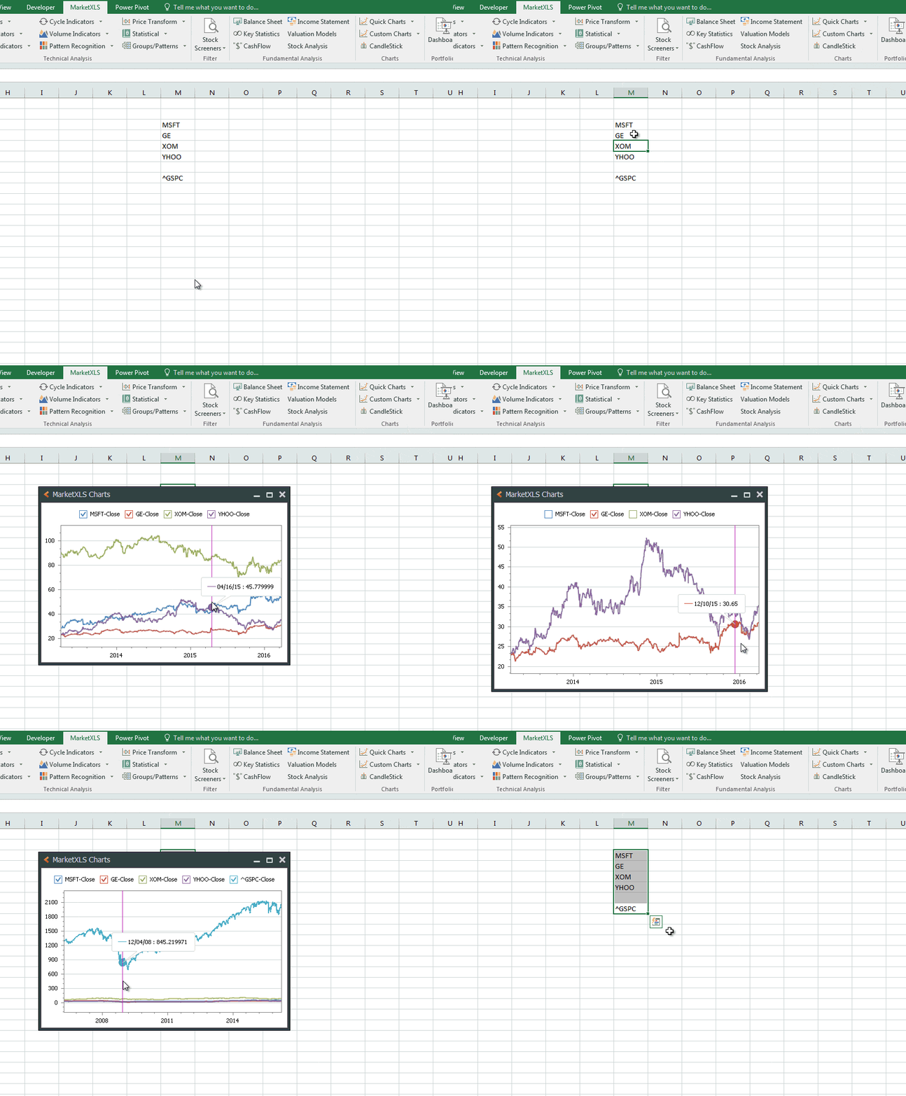
Are you tired of having to log into your stock brokerage account to check your portfolio balance? Or maybe you are looking to do some technical analysis using live stock quotes? Without a doubt there are a lot of solutions out there. But most of them are not as straightforward as MarketXLS.

MarketXLS is a one stop solution for technical and fundamental analysis. With MarketXLS you can do research (technical, fundamental and options) the way you like in Excel.

Simple Pricing, No Surprises

24/7 customer service. One Time Pricing. 

Immediate Download and License Delivery 

30 Day Money Back Guarantee

Download now with coupon code: StockKevin and save 20%.

Stock Charts in Excel

- Ready made stunning stock charts in Excel 

- Make your own charts with any dataset in Excel

- Zoom in – Zoom out of charts with dynamic dates handling

- Exports charts in multiple formats

- Annotate Candlestick patterns on chart

- Auto-identification of data series, no settings needed

- Maximize chart windows without distortion of clarity

- Open multiple charts in Excel at a time

- Much more interactive and dynamic than native charts in excel

[Continue reading...]

MarketXLS Review : Pull Stock Quotes and Perform Fundamental and Technical Analysis within Excel

We are constantly looking for ways to analyze stock prices.

There are two ways to pull stock quotes into a readable and analyzable format. We've documented steps on how that can be done through Microsoft Excel or Google Sheets. There are major pros and cons with using either. For example, with Excel you don't need to be connected to an internet browser, but the functionality is limited and bulky. The blue bars are an eye sore. In Google Sheets, you'll need to open up a browser. But, at least it is nice and clean.

What if you had a way to combine the best of both Excel and Google Sheets worlds and increase functionality. Just a couple weeks ago, a friend of mine introduced me to an excel plug-in called MarketXLS. Is is a software that is directly downloadable instantly over the web. It pulls quotes into your Excel sheet using formulas that pull real-time quotes seamlessly.

One of the most useful and used formula is the "=ask("TICKER")". Simply type in =ask("WFM") and it will pull in the ask price instantly.

One of the best things about marketXLS is the fact that you can pull in historical stock data. We are constantly looking for ways to analyze stock prices and compare them to 52-week lows or just looking at technical trends. The software pulls reliable data from Quotemedia and can provide minute by minute data updates. 

What if you had a way to combine the best of both Excel and Google Sheets worlds and increase functionality. MarketXLS does just that.

If I was doing technical analysis, MarketXLS provides a number of indicators and analysis that would be extremely helpful. Personally, there are just too many for me to really grasp. However, you might find use in them if you are looking to do find a hammer pattern or a gravestone doji. 

Personally, I prefer fundamental analysis and stock screening tool. MarketXLS is able to pull in actual income statements, balance sheets, and cash flows. This is especially important when you are analyzing how much a company is returning on its tangible assets. Being able to pull these directly into your excel without having to visit the SEC website is definitely a time saver. Right now it is able to pull in three years, however it would be nice if it could pull in five years of data. 

I want to point out that under the "Utilities" tab you can pull in dividend history information, which is really cool. It is one less step to having to pull information from a browser. I literally place my mouse on a cell with the stock ticker and click on "Dividend History" and all of that dividend history gets pulled in to my Excel like magic.

How do you screen for stocks or find stocks to buy?

MarketXLS allows you to screen stocks based on cash flow ratios, balance sheet items, profitability, gross margin, and even more things including return by period. 

Note that the above is a real review of the product paid for by our sponsored partner. 

[Continue reading...]

Excel Tip #17 - Shortcut to Naming Cells or Ranges and Why You Should Name Excel Cell Ranges

Suppose you have a 5x5 Microsoft Excel table. On the top row you have the months of the year beginning with January through May. Then on the left hand side you have stock ticker symbols including but not limited to AAPL, GOOGL, and WFC. In the heart of all of this you have the stock prices of the respective month and ticker.

Your goal is to find the average price for GOOGL in the five months beginning in January.

The simple answer would be to type in the =average formula and drag your mouse over the row beginning with GOOGL. Maybe you are somewhat more Excel savvy and directly type in =average(D5:H5) instead.

Let me introduce to you a third, more efficient and flexible method. Suppose you name that range from D5:H5 "GOOGL". Going forward all you have to do is type in =average(GOOGL). If you are adding more months just make sure you include the additional months in the cell name.

Now, it is quite easy to highlight five cells and type in "GOOGL" in the box to the left of your formula toolbar.

If you have a table that is 100x100, that can become tedious. What is an easy and quick shortcut to naming all of the columns and rows with their headers?

The answer is to highlight the table and hold CTRL+SHIFT+F3 to name the columns and rows based on headers. You will be prompted with the 'Create Names from Selection' box. The default is the 'Top Row' and 'Left Column'. In our example, this means the columns with header 'Jan' will be named 'Jan' and the row 'AAPL' will be named 'AAPL'.

Let's say that you forgot what cells ranges in Excel you named and don't want to duplicate names. Hit CTRL+F3 and you will see all the cells and cell ranges you've named already along with which cells are being selected as part of that name tag.

Quick Summary

1) Quickly sum cell ranges using the cell name in replacement of the cell range
2) Highlight table and hold CTRL+SHIFT+F3 to name the columns/rows based on headers
3) Use shortcut CTRL+F3 to bring up the 'Name Manager' to view named cells ranges

For more excel tips check out the #1 best selling e-commerce book below.

[Continue reading...]

Excel Tip #16 - Filling in Blank Cells with Header Cell Values

Excel - Fill in those Blank Cells with Header Information

When you have a report that has some of the header information filled out but not all of it, what is the best way to fill in blank cells with header values? 

This is especially the case when the rows in your report have repeating information. Typically, the report itself will just show the first new value and leave the remaining blank. This is great if you are viewing the report because you don't want extraneous information. But, what if you want to sort the information and organize a pivot table? You'll need to manually type in the blanks, but that could take you a couple of hours. Imagine if you had thousands of pages of blanks, that would take you days. 

This five step process will help you fill in the blanks with header cell values within minutes! 

1. Highlight and select the range with blanks, including headings to be copied. 

2. Hit "F5", which will prompt up the "GoTo" dialog box.

3. You'll want to hit "Special" and select "Blanks". Then hit "OK".

4. Press "=" key and the Up Arrow.

5. Hold down the Control key and press Enter.

[Continue reading...]

Excel Tip #15 - Macro to Pull Information from One Excel Workbook into Another

In accounting sometimes we download GL detail from the accounting system or pull information from a third-party source and then we dump that data into an excel workbook. Often times that information is used in multiple excel workbooks. But it becomes cumbersome when you have to manually copy and paste that information from one spreadsheet to another. Why not just have a macro do it for you? Yes, we've created a macro that will copy data from one spreadsheet (doesn't have to be open) into another spreadsheet instantly.

Here is the solution. Though you will need to make some changes to the code below.

a] Get_Copy_Data - This is what you want to name your macro. Leaving it as is will not affect the code.

b] CopyDataSheet - This is the name of the sheet you would like the data copied to.

c] C:\Users\z3n\Desktop\hapy.xlsx - This is the file path of the excel workbook that already has the data. Make sure it is in the first tab.

d] hapy.xlsx - This is the excel workbook that has the data already

1) Hit Alt + F11 (this will open the VBE Window)
2) Select 'Module' from the 'Insert Menu' and paste the code below.

 Sub Get_Copy_Data()
    Sheets("CopyDataSheet").Select
    Range("D7").Activate
    Selection.ClearContents
ThisWorkbook.Activate 'start in THIS workbook
 Sheets(1).Select 'switch to data import sheet
'Opens source file (this filename never changes)
 Workbooks.Open Filename:="C:\Users\z3n\Desktop\hapy.xlsx", ReadOnly:=True
Workbooks("hapy.xlsx").Activate 'switch to source workbook
 Sheets(1).Select 'switch to source data sheet
 [a1].CurrentRegion.Copy 'Copy data to clipboard
ThisWorkbook.Activate 'Return to THIS workbook
[G7].PasteSpecial Paste:=xlPasteValues 'paste data to import start cell
[a1].Select 'cancels highlighted paste region
Workbooks("hapy.xlsx").Close 'close source data workbook
Sheets("CopyDataSheet").Select
    Range("A1").Select
    ActiveSheet.Paste
End Sub

At the moment, you'll have to save this in your "Personal" macro book. It has trouble when you save the macro in the workbook itself.  

[Continue reading...]

Excel Tip #14 - Exclude Certain Criteria in SUMIF and SUMIFS

Suppose you want to sum a bunch of numbers, but only if they meet certain criteria. One way to do this is manually in Excel. Say we want to find 'GL' account 102015 with the 'Dimension' 5 and sum the 'Total Balance' of that. In the below example the total would just be 35.

This is simple enough to do when you only have a list of less than 10 items. Suppose you are dealing with large data sets with more than a thousand lines. It can get tedious to sum all the 'Total Balance' with the two above criteria.

Introducing SUMIF and SUMIFS Formulas

=SUMIFS(C3:C9,A3:A9,102015,B3:B9,5)

This formula above is telling Excel to sum the 'Total Balance' column (C3:C9) if both the 'GL' column (A3:A9) and 'Dimension' column (B3:B9) equal 102015 and 5 respectively. The total is 35.

However, suppose instead you want to sum everything EXCEPT 'GL' column with 102015 and 'Dimension' with 5. One way of doing this is by adding criteria after criteria in the above function. This would mean a longer excel formula. You can do this by adding the 'Criteria Range' and then the 'Criteria'.

=SUMIFS('Sum Range', 'Criteria Range1', Criteria1, Criteria Range2, Criteria2, Criteria Range3, Criteria 3,)

Formula to the Excluding Certain Criteria

=SUMIFS(C3:C9,A3:A9,"<> 102015",B3:B9,"<> 5")

This formula will sum everything in the 'Total Balance' column that does not meet the criteria of a GL 102015 and Dimension 5. Alternatively to only exclude one criteria you can easily just enter in SUMIF(Range, Criteria, Sum Range) whereby the 'Range' is the column with the 'Criteria' you are looking to exclude and 'Sum Range' is the balances you want to sum.

[Continue reading...]

Excel Tip #13 - Easily Transpose a Data Set (Flip data from horizontal to vertical or vice versa)

Four Steps to Paste Special Your Way to Transposing Data

Some tables are best looked at with the headers going across versus on the left side. Suppose you've always labeled your table with column headers versus row headers, but now you want to swap it and have the headers go on the left side versus across on top. There are two easy ways of doing this. One is through the below simple four step process. The other is through pure shortcuts. Take your pick.

1. Select range to be transposed
2. Ctrl +C or Copy Button
3. Select the Paste Cell
4. Right Click, Choose Paste Special, Transpose

Super Pro Tip:

Hit: Alt then, E, S, V, E and then click 'Ok'

[Continue reading...]

Excel Tip #11 - Find Your Document File Path URL

Where is the File Path for my Excel workbook?

How many times has your colleague asked you to send him or her the file path of a file? In accounting, this happens so often when we have to review each other's work. When you have thousands of excel files in various folders it gets hard to keep track of where things are. Instead of going through your files and trying to type out your file path of C:\Users\My Computer\File, why not just put it in your Excel Quick Access Tool Bar.

Here is how you can find the file path of your excel workbook. 

1) Go to 'File' in the top left corner of your excel program. 

2) Simply click on 'Options' -> Quick Access Toolbar -> Sort by 'All Commands'

3) Find the 'Document Location' -> Add >>

Then it should show up on your ribbon and now all you have to do is copy and paste that location and email it to your colleague or whomever. Simple as that!

[Continue reading...]

Excel Tip #10 - Change a Single Spaced Sheet into a Double Spaced Spreadsheet

Three Step Process to Instantly Adding a Space Between Rows in a Table

Within Excel, there is more than one way of adding spaces between row in a data set. We can manually add blank rows or we can use a shortcut such as holding Ctrl Shift and +. These two methods are absolutely acceptable if you only have a couple of rows. But what if you had a hundred or a thousand rows? It would take you a long time to change your single spaced sheet into double spaced. Luck for you, there is a more efficient way to do this. 

Suppose your end goal is illustrated below (ignore column F for now). You want each row of data to be separated by a blank space. This could be because you want your data to look cleaner or just easier to read. 

You started with the below data set. One way of spacing this out is by adding numbers to the right or left side of the data set. In the below spreadsheet picture, we've labeled each row of data from one to eight. Then just below it repeat the same numbers. 

After you've finished labeling the rows as such, find the filter button which is under 'Sort & Filter'. You can then either sort from smallest to largest or largest to smallest. Depending on how you sort, your list could be flipped or remain the same. Pick smallest to largest and if that is how you labeled it, then it will look as if you just add extra rows to your original data set. 

After that you should get your double spaced spreadsheet. You can now delete the column you added and your sheet will still be spaced. And that is how you change a single spaced sheet into a double spaced spreadsheet!

[Continue reading...]

Excel Tip #9 - Pull Number or Text from the Middle of Text String

Excel - Extract Certain Characters from Text String

As accountants, we constantly deal with the general ledger. Most of the general ledger (GL) reports we run either from Oracle, Microsoft AX, or Quickbooks contain long text strings.

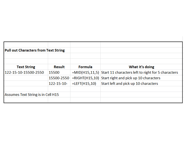
For example, if I have a company account 122, subsidiary 15, product line 10, general ledger account 15500, and sub-ledger/other random number of 2550 my text string would look like 122-15-10-15500-2550.

That text string is extremely annoying especially if all I want to do is sort in excel by a particular general ledger account. Say I wanted to sort by GL#15500, but my beginning strings are all different. For example, I have company account 122, 133, 145, and 166. It would be difficult to sort just by my general ledger account 15500.

What is your solution to extracting numbers from text strings?

Try the following formula =MID(text, start_num, num_chars). 

1) For "text", select the cell where your text resides. The one you want to pull the number from.

2) "start_num" refers to where you want the pulled number to start from left to right. So if my text string is 122-15-10-15500-2550. The 11th text (including dashes) is my general ledger account.

3) "num_chars" refers to how many characters I want to pull beginning from my "start_num". In this case it would be 5.

My formula for the above text string would be =MID(H15,11,5). The result is 15500. 

What if I wanted to just pull text from the right or the left?

Use =LEFT(text, num_chars) or =RIGHT(text, num_chars).

This will pull the number of characters beginning from the left for LEFT and right for RIGHT.

[Continue reading...]

Excel Tip #8 - How to Put Random Numbers in Excel?

Why would you ever want to put random numbers in excel?

As an auditor, you make test selections from large sample of data. For example, if you were looking to test revenue transactions, you want to make sure that revenue actually exists, is accurate, occurred in the proper period, etc.

You might get a detailed listing of all revenue transactions for the quarter and pick a couple selections to "follow" the transaction through or obtain support for. This revenue listing could be thousands of excel pages long. You would probably need some way to pick your samples.

With a random number generator you would be able to do just that. You can randomly assign each selection with a number and then sort by that number. This would give you a list of randomly selected sample sizes. Alternatively, if you were looking to randomize the list, assigning a number would also work.

Here are the formulas for generating random numbers.

=RAND() - For random number between 0 and 1

=RAND()*100 - For random number greater than or equal to 0 but less than 100

=RANDBETWEEN(low,high) - For a random integral number between the high and low number. Fill in low and high with your desired range. For example, =RANDBETWEEN(5, 100) would give you numbers between 5 and 100.

[Continue reading...]

Excel Tip #7 - Shortcut to Deleting Multiple Blank Rows in Workbook or Sheet

Deleting Blank Rows Should Not Be a Manual Process

Recently, I copied over a list of colors in Spanish from Microsoft Notepad. Of course, after I copied it over, it left a bunch of blank spaces and rows. Now, my list here isn't that bad. But if I had a longer list it would be a pain to manually delete them one by one.

In theory, I could just select each row and then right-click -> Delete -> Entire row.

Alternatively, I could select a cell in the row and then press and hold "Ctrl" and "-" signs. 

Personally, if I have a long list of blank rows and it is separated by rows with text, all of the above two methods take too much time.

Here is a four step approach to deleting multiple blank rows in the workbook in one scoop. 

1) Select the columns with the blanks. 

2) Press F5 to bring up the "Go To" box. Then press and hold ALT and S or just select "Special...".

3) Press and hold ALT and K or select "Blanks".

4) Press and hold Ctrl  and - signs to delete and shift the cells up

There you go! Now you've saved a bunch of time!

[Continue reading...]

Excel Tip #6 - How to Count or Sum All the Positive/Negative Numbers in a Row/Column

Excel Formula - Count or Sum All Positive or Negative Numbers in a Row or Column

As mentioned in Pro Stock Trading Tips #1, it is essential for the trader to let gains run and cut losses.

One way of tracking whether or not you are doing this is by actually looking at your trading results. If you track your results in excel, there are simple formulas you can employ to count the number of winners or losers you have and how much the total of your winners or losers is.

Counting number of positive or negative numbers use: 

a) Number of all positive numbers

=COUNTIF(D5:D20,">0")

b) Number of negative numbers

=COUNTIF(D5:D20,"<0")

Replace D5:D20 with your actual data set.

Summing all the positive or negative numbers separately use:

a) Sum of all positive numbers

=SUMIF(D5:D20,">0")

b) Sum of negative numbers

=SUMIF(D5:D20,"<0")

Again, replace D5:D20 with your actual data set. 

Average all the positive or negative numbers use:

a) Average of all positive numbers

=AVERAGEIF(D5:D20,">0")

b) Average of all negative numbers 

=AVERAGEIF(D5:D20,"<0")

For examples of this see Pro Stock Trading Tips #1 where an excel screenshot has been included. Be sure to replace the D5:D20 to your actual data set.

[Continue reading...]

Ultimate Running List of All Helpful Microsoft Word/Excel Shortcuts & Formulas

The one thing all of us wish we had more of is time. Technology has helped us perform tasks that used to hours in minutes. But we all know that when we have to troubleshoot, it can take days.

Here is a list of all the helpful Microsoft Word/Excel shortcut that can help you save time here and there. I will continue to update this list as I think of shortcuts and formulas.

Microsoft Word

Ctrl+Alt+M = Add comment box


Microsoft Excel

Ctrl+Shift + "+" = Insert row or column/ Shift cells left or right
Shift + F2 = Insert a comment in a cell
Alt + R + D = Deletes comment in a cell
Ctrl + 1 = Open up the 'Format Cells' box

Formulas

To automatically calculate the day of the week.
Enter a date reference in cell A2
Enter =TEXT(WEEKDAY(A2), "ddd") into the cell in which you want the day to appear.

[Continue reading...]

Excel Tip #4: Investment Banking and Big 4 Accounting Bare Minimum Excel Basics

In the investment banking industry, analysts and associates are expected to use excel without a mouse. How is that possible you ask? The below excel tips can help you with that. These are the basic fundamental excel hot keys that will help you navigate throughout your excel sheet without a mouse.

Though it is not necessary in Big 4 accounting, it does save you time. You will appreciate these tips in January through March when you are in the busy season.

1. Move from your selected cell to the last cell either by row or column. 
Hot Keys : Hold Ctrl and use the directional keys (left, right, up, or down) 
Comments: If there is data in the cells, this will take you to the last cell with data either by row or column. However, if there is an empty cell in that row or column, this will take you to the first cell after the last empty cell.

2. Highlight from your selected cell to the last cell either by row or column.
Hot Keys: Hold Ctrl and shift then use the directional keys (left, right, up, or down)
Comments: Same rules apply as the shortcut above except instead of jumping to a cell, this highlights it.

3. Add an additional column or row 
Hot Keys: Hold Ctrl and shift then press +
Comments: From the "insert" box select whether or not you want to add the 'Entire row' or 'Entire Column'. Pressing "r" and hitting 'Enter' adds entire row. Pressing "c" and hitting 'Enter' adds an entire column.

4. To use the toolbar at the top 
Hot Key: Hit Alt 
Comments: This will highlight all the functions at the top. Then it is a matter of time before you familiarize yourself with the different hot keys to navigate within the above toolbar. For example, if you hit "Alt" then "r" and finally "c" then you will add a comment box. 

5. To view/alter a cell's formula
Hot Key: Hit F2 
Comments: Additional tip for creating absolute functions - Hit F4. This will help you cycle through a number of formulas. Remember the $ means that the coordinate is absolute even as you drag the formula across cells or copy the formula into another cell. 

6. Trace back a formula into another cell or tab. 
Hot Key: Hold Ctrl and then press [ 
Comments: This is particularly useful in determining where the formula is pulling from and prevents the need of toggling back and forth just to see where the formula is pulling from.

[Continue reading...]

Windows Quick Tips Shortcuts

This isn't necessarily an Excel Tip, but this is still helpful.

Anything to shave a couple seconds from your work day. Of the below, I use the 'windows key + M' shortcut the most.

1. Ctrl + Drag File
Makes a quick copy of the file/folder

2. Windows key + M
Minimizes all open windows

3. Alt + double click file/folder
Pulled up the 'System Properties' dialog box

[Continue reading...]

Excel Tip #3: Why does my VLOOKUP return #N/A?

VLOOKUP FAIL 

Have you ever had an Excel formula not work, but you've checked the formula multiple times already? You are certain that the formula is correct, but excel returns back #N/A or a blank. Do you wonder what is going on?

Due to Excel's stupidity, the format of your data you want returned has to match the format of the data you are pulling from. From this is not the case, your vlookup will return a bunch of retarded #N/As or blanks.




For example, let's say you are looking for the purchase order 6555 in the table below, and you want to return the amount from column 3 of that table. For one reason or another you may have extracted the below information from a PDF by saving it into notepad and then using the Text to Excel conversion to convert it to Excel. Somewhere along the way the format of the data went haywire.

Today is your lucky day, there is a solution. Find a blank cell and type in any number. Then copy the cell and paste special over the problem cells using past 'values' and 'multiply. Now the number that Excel though was just text (or some other crap) is now a number that vlookup understands.

[Continue reading...]

Excel Tip #2: How to Set Up an Automated Table of Contents in Microsoft Word

Three step process to setting up an automated table of contents in Microsoft Word

1) Type in the document the “title” (Prologue) of the first page of your table of contents

2) Highlight the title and click on the “Home” tab, in the “Styles” section select “Heading 1”

3) Click outside of your “title” and click on the “References” tab, in the “Table of Contents” section select “Table of Contents”

Poof! You should have something like this:

Contents
Prologue....................................................................................................................................1

[Continue reading...]

Excel Tip #1 - Copy/Paste Sum of Selected Cells

How to Copy/Paste the Sum of Selected Cells in Excel

I've booked about three hundred hours plus of work in March. This is not by choice, it's just the nature of the business, but I am always looking for ways to be more efficient. As an auditor, there are a lot of menial tasks that can be eliminated with macros in excel files. We are interested in totals and it's a pain to have to copy a set of numbers into another worksheet and sum them up to get the number you need. Typically when you highlight a set of numbers the total will appear on the bottom left hand corner. I wanted to be able to copy that total directly and paste it in a separate spreadsheet.

Here is a macro that will help you do that.

Refer to the below five step process:

1) Hit Alt + F11 (this will open the VBE Window)

2) Select 'Module' from the 'Insert Menu' and paste the code below.

Sub mySum()
Dim MyDataObj As New DataObject
MyDataObj.SetText Application.Sum(Selection)
MyDataObj.PutInClipboard
End Sub

3) Select 'References' from the 'Tool Menu' and make sure 'Microsoft Forms 2.0 Object Library' is selected. If it's not listed then click 'browse' and select 'Fm20.dll'

4) Close the VBE window

5) Hit Alt + F8, select 'mySum', click 'Options' and set your shortcut key.

[Continue reading...]